という質問を受けた。
結論から言うとおかしくない。メタアナリシスのweight は各研究内の分散
と研究間の分散
により
(fixed model の場合)もしくは
(random effect model の場合)
で決まるから、分散が小さい、すなわち推定精度の高い研究はweight が大きくなる。サンプルサイズが大きいと推定精度が増すので、サンプルサイズが大きいことがweight を大きくする要因だが、分散がそもそも小さいことも重要である。
とあるメタアナリシスで、サンプルサイズが114+115のKienast という研究(29%)より、サンプルサイズが33+23のBaudoという研究(57%)のほうがweight が大きい。
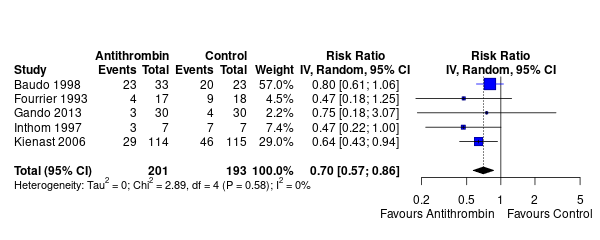
Baudo の研究だけ取り出してみると、分割表は
であるが、周辺度数を固定したときに、この分割表の取りうる運命は、 を変動させて
となる。
を変動させて、そのときの分割表のMH検定を行い、信頼区間の幅を見てみると、
のときに信頼区間の幅が最小になる。すなわち、推定の精度がよいことになる。
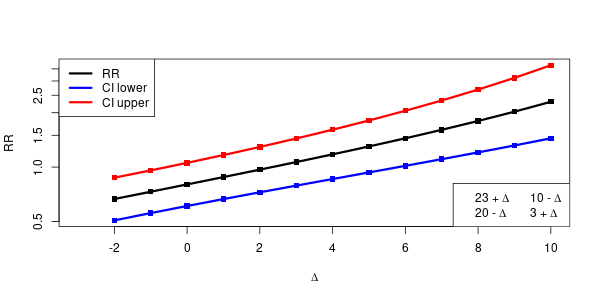
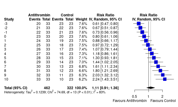
すべての の取りうる範囲が、各々メタアナリシスに組み入れられた研究だと仮定して、それら全体をメタアナリシスしてみる。確かに、信頼区間の幅の狭い
などの研究が、weight が大きい、ということになっている。
library(meta)
library(epiR)
library(latex2exp)
# 元のデータ
dat <- cbind.data.frame(
   author=c("Baudo", "Fourrier", "Gando", "Inthom", "Kienast"),
   year=c(1998, 1993, 2013, 1997, 2006),
   ev.exp=c(23, 4, 3, 3, 29),
   n.exp=c(33, 17, 30, 7, 114),
   ev.cont=c(20, 9, 4, 7, 46),
   n.cont=c(23, 18, 30 ,7, 115)
   )

cols <- replace(rep("black", nrow(dat)), dat$author=="Baudo", "blue")

m <- metabin(ev.exp, n.exp, ev.cont, n.cont,
             method="Inverse",
             data=dat, studlab = paste(author, year),
             label.e="Antithrombin", label.c="Control",
             label.right="Favours Control", col.label.right="red",
             label.left = "Favours Antithrombin", col.label.left="blue")

forest(m, col.study=cols, layout="RevMan5", comb.fixed=FALSE)

# Gando に着目する
i <- 1
b <- rbind(c(dat[i, "ev.exp"], dat[i, "n.exp"]-dat[i, "ev.exp"]),
           c(dat[i, "ev.cont"], dat[i, "n.cont"]-dat[i, "ev.cont"]))

# MH test
A <- matrix(c(1, -1, -1, 1), 2)
r <- epi.2by2(b, method="cohort.count")
r$massoc$RR.strata.taylor

# Delta をすべて動かして検定する
x <- (-sort(b)[1]):(sort(b)[2])
bs <- mapply(function(z) b + A*z, x, SIMPLIFY=F)
r <- mapply(function(z) try(unlist(epi.2by2(z)$massoc$RR.strata.taylor)), bs, SIMPLIFY=FALSE)
g <- t(mapply(function(z) switch(any((is(z)%in%"try-error"))+1, z, rep(NA, 3)), r))
g <- matrix(unlist(g), nrow(g))
colnames(g) <- c("RR", "CI lower", "CI upper")

cols <- c("black", "blue", "red")
txt <- mapply(function(z, w) substitute(x~y~Delta, list(x=z, y=w)), c(b), c("+", "-", "-", "+"))
matplot(x, g, type="o", pch=15, lty=1, xlab=expression(Delta), ylab="RR", col=cols, lwd=3, log="y")
legend("topleft", legend=colnames(g), col=cols, lty=1, lwd=3)
legend("bottomright", legend=sapply(txt, as.expression), ncol=2)

# すべてのDelta に対応する分割表が各研究だとみなしてメタアナリシスする
bs1 <- sapply(bs, c)
bs0 <- cbind(bs1[1,], bs1[1,]+bs1[3,], bs1[2,], bs1[2,]+bs1[4,])
colnames(bs0) <- tail(colnames(dat), 4)
bs0 <- cbind.data.frame(year=x, bs0)
m <- metabin(ev.exp, n.exp, ev.cont, n.cont,
             method="Inverse",
             data=bs0, studlab=year,
             label.e="Antithrombin", label.c="Control",
             label.right="Favours Control", col.label.right="red",
             label.left = "Favours Antithrombin", col.label.left="blue",
             )

forest(m, layout="RevMan5", comb.fixed=FALSE)